Seismic Surveys

Seismic surveys use low frequency acoustical energy generated by explosives or
mechanical means. These waves travel downward, and as they cross the boundaries
between rock layers, energy is reflected back to the surface and detected by sensors called
geophones. The resulting data, combined with assumptions about the velocity of the
waves through the rocks and the density of the rocks, are interpreted to generate maps of
the formations.
Seismic surveys are usually performed using multiple geophones set at known distances
from the energy source. Early seismic surveys used mechanical plotters to record the
received signals, and were restricted to a few geophones. These surveys placed the source
and geophones in a straight line, with the interpretation of the resulting data producing a
2-D cross section of the formation under that line. The interpretations were subject to
error, which increased the difficulty, and cost, of accurately locating hydrocarbon-bearing
formations.
Today, the development of digital recording systems allow the recording of data from
more that 10,000 geophones simultaneously, greatly speeding data collection.
Sophisticated computer programs develop highly accurate 3-D models of rock structures.
These models are more accurate than past 2-D maps, and increase the likelihood of
accurately identifying hydrocarbon-bearing formations.
Seismic Section
The seismic reflection method works by bouncing sound waves off boundaries between
different types of rock. The reflections recorded are plotted as dark lines on a seismic
section. A seismic section resembles a geological cross-section, but it still needs to be
interpreted.
One major difference between a geological cross-section and a seismic section is that the
vertical axis is in time, rather than depth. In the earth's crust, seismic waves travel
typically at about 6000 m/s so that 1 second of two-way travel time corresponds to about
3 km of depth. All the seismic sections presented in this atlas are plotted at 1:1 (no
vertical exaggeration) assuming an average crustal velocity of 6000 m/s.
Another difference is that the reflections are plotted halfway between the source and the
receiver. These are referred to as unmigrated data. The process that moves the reflections
in their correct spatial position is referred to as migration, and the resulting seismic
section is referred to as a migrated section.
The science of LITHOPROBE is spearheaded by the seismic reflection method because it
is the geophysical technique which produces the best images of the subsurface. These
data resolve mappable features such as faults, folds and lithologic boundaries measured
in the 10's of meters, and image them laterally for 100's of kilometers and to depths of 50
km or more (Varsek, 1992).
Seismic reflection profiling is the principal method by which the petroleum industry
explores for hydrocarbon-trapping structures in sedimentary basins. Its extension to deep
crustal studies began in the 1960s, and since the late 1970s reflection technology has
become the principal procedure for detailed studies of the deep crust.
Seismic data acquisition
The method works by bouncing sound waves off boundaries between different types of
rock (Figure 1). As opposed to earthquake seismology, where the location and time of the
source is an unknown that needs to be solved for, seismic reflection profiling uses a
controlled source to generate seismic waves. On land, LITHOPROBE has been using
large truck-mounted vibrators as a source (the "Vibroseis" method), and occasionally
dynamite is used. At sea, large arrays of airguns, which rapidly eject compressed air, are
deployed. The reflected signals are recorded by geophones, or hydrophones at sea, which
resemble ordinary microphones

. 

                                                      Figure 26 – Seismic data Acquisition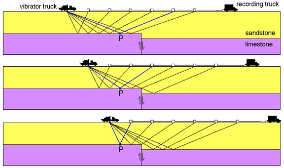

During a seismic survey, a cable with receivers attached to it at regular intervals is laid
out along a road or towed behind a ship. The source moves along the seismic line and
generates seismic waves at regular intervals such that points in the subsurface, such as
point P in Figure 1, are sampled more than once by rays impinging on that point at
different angles. As a shot goes off, signals are recorded from each geophone along the
cable for a certain amount of time, producing a series of seismic traces. The seismic
traces for each shot (called a shot gather) are saved on magnetic tape in the recording
truck.
Seismic data processing
Digital data processing is applied to raw seismic data to produce a seismic section (Figure

27). The following is an example of typical processing sequence.

Figure 27. Seismic data processing.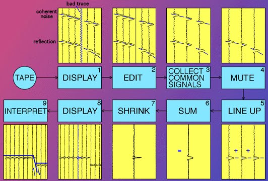
The data are read from tape and the shot records (i.e. all traces recorded for a given shot)
are displayed (1). Bad seismic traces, due to noise or a short circuit in the recording
equipment, are edited out (2). The traces are then reordered (3) so that each gather of
traces belongs to a common reflection point, such as point P in Figure 26.
Non-reflected arrivals, such as surface waves and direct arrivals, are removed by digital
filtering and/or muting (zeroing of the data) (4). A correction is made for the time the
reflected ray spends travelling laterally, so that the reflected arrivals now line up (5).
These traces are then added to produce a single output trace (6). This process, referred to
as stacking, cancels out random noise and reinforces the reflected signals. The waveform
is then shrunk by frequency filtering or deconvolution to improve the resolution (7).
Steps (4) to (7) are repeated for each common reflection point, and the resulting seismic
traces are displayed as a seismic section (8) which is then interpreted (9).